Basic Concepts#
Probability Basics#
Probability of an Event:
Conditional Probability:
Bayes’ Theorem:
Law of Total Probability:
Random Variables#
Expected Value:
(for discrete)
(for continuous) 2. Variance:
Standard Deviation:
Common Distributions#
Binomial (n trials, p success probability):
Poisson (λ rate):
Normal (μ mean, σ standard deviation):
Descriptive Statistics#
Mean:
Sample Variance:
Correlation:
Inferential Statistics#
Z-Score:
t-Score (for sample):
Regression#
Simple Linear Regression:
OWLS#
06/10/2023 The equation \( \mathbf{w}^* = (\mathbf{X}^T \mathbf{X})^{-1} \mathbf{X}^T \mathbf{y} \) is the solution for the weights \( \mathbf{w}^* \) in linear regression using the method of least squares. Let’s break down how we arrive at this solution:
Derivation of the Optimal Weights in Linear Regression (OWLS第一万遍): Regression Modelling And Least-Squares
Objective:
In linear regression, we aim to minimize the sum of squared residuals (SSR), which is the difference between the observed values (\( \mathbf{y} \)) and the predicted values (\( \mathbf{Xw} \)).
The objective function (SSR) is given by:
\[ SSR(\mathbf{w}) = (\mathbf{y} - \mathbf{Xw})^T (\mathbf{y} - \mathbf{Xw}) \]
Differentiating with Respect to \( \mathbf{w} \):
To find the weights that minimize the SSR, we differentiate the SSR with respect to \( \mathbf{w} \) and set the result to zero. This will give us the weights that minimize the SSR.
Differentiating, we get:
\[ \frac{\partial SSR}{\partial \mathbf{w}} = -2\mathbf{X}^T (\mathbf{y} - \mathbf{Xw}) \]
Setting the Gradient to Zero:
For the minimum, we set the gradient to zero:
\[ -2\mathbf{X}^T (\mathbf{y} - \mathbf{Xw}) = 0 \]This simplifies to:
\[ \mathbf{X}^T \mathbf{y} = \mathbf{X}^T \mathbf{Xw} \]
Solving for \( \mathbf{w}^* \):
To isolate \( \mathbf{w} \), we multiply both sides by the inverse of \( (\mathbf{X}^T \mathbf{X}) \):
\[ \mathbf{w}^* = (\mathbf{X}^T \mathbf{X})^{-1} \mathbf{X}^T \mathbf{y} \]
This solution provides the optimal weights for a linear regression model in the least squares sense. It’s worth noting that this solution assumes that \( (\mathbf{X}^T \mathbf{X}) \) is invertible. If it’s not (e.g., in cases of multicollinearity), then additional techniques or regularization methods might be needed.
Fisher Info#
Fisher Information Matrix (FIM)第一万次:
Definition:
For a single parameter \( \theta \), the Fisher Information \( I(\theta) \) is defined as the variance of the score, which is the derivative of the log-likelihood:
\[ I(\theta) = \text{Var}\left( \frac{\partial \log p(x|\theta)}{\partial \theta} \right) \]For multiple parameters, the Fisher Information Matrix is defined as:
\[ I_{ij}(\theta) = E\left[ \frac{\partial \log p(x|\theta)}{\partial \theta_i} \frac{\partial \log p(x|\theta)}{\partial \theta_j} \right] \]where the expectation is taken over the distribution of the data \( x \).
Interpretation:
The FIM quantifies how much information the data provides about the parameters of the model.
Larger values in the FIM indicate that small changes in the parameter \( \theta \) would result in larger changes in the likelihood, meaning the data is more informative about that parameter.
Properties:
Invertibility: The inverse of the FIM (if it’s invertible) provides a lower bound on the variance of any unbiased estimator of the parameter \( \theta \). This is known as the Cramér-Rao bound.
Additivity: For independent observations, the Fisher Information is additive. That is, the information from each observation can be summed up.
Applications:
Parameter Estimation: The FIM is used in the context of the Cramér-Rao bound to determine the minimum variance (best precision) that can be achieved by an unbiased estimator.
Experimental Design: In experimental settings, the FIM can be used to design experiments that maximize the information about parameters of interest.
Model Comparison: Models can be compared based on the amount of information they provide about parameters or underlying processes.
Connection to Linear Regression:
In the context of linear regression with Gaussian errors, the Fisher Information matrix is proportional to \( \mathbf{X}^T \mathbf{X} \), where \( \mathbf{X} \) is the design matrix. This relationship is particularly clear when considering the maximum likelihood estimation in linear regression.
In essence, the Fisher Information Matrix is a measure of how sensitive the likelihood function is to changes in the parameters. It plays a crucial role in understanding the precision and reliability of parameter estimates in statistical models.
Certainly! Let’s use a simple example to illustrate the concepts of incorporating prior beliefs and uncertainty quantification in Bayesian linear regression.
07/10/2023
Multivariate Gaussian#
(PP 6.1) Multivariate Gaussian - definition
14/10/2023
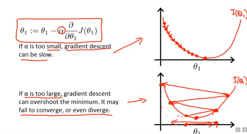
Learning Rate#
Gradient Descent, Step-by-Step
In gradient descent, the learning rate represents the size of the steps taken during each parameter update and affects the trade-off between convergence speed and stability of the optimization process.
Learning rate is a hyper-parameter that controls how much we are adjusting the weights of our network with respect the loss gradient.
Absolutely, the concept of hidden layers can be abstract and sometimes confusing, especially when you’re first getting into deep learning. Let’s break it down:
17/10/2023
Conclusion:#
In essence, hidden layers can be seen as a series of transformations that refine and process the input data to produce an output. They enable deep learning models to capture intricate patterns and relationships in the data, making these models powerful tools for a range of tasks.
18/10/2023
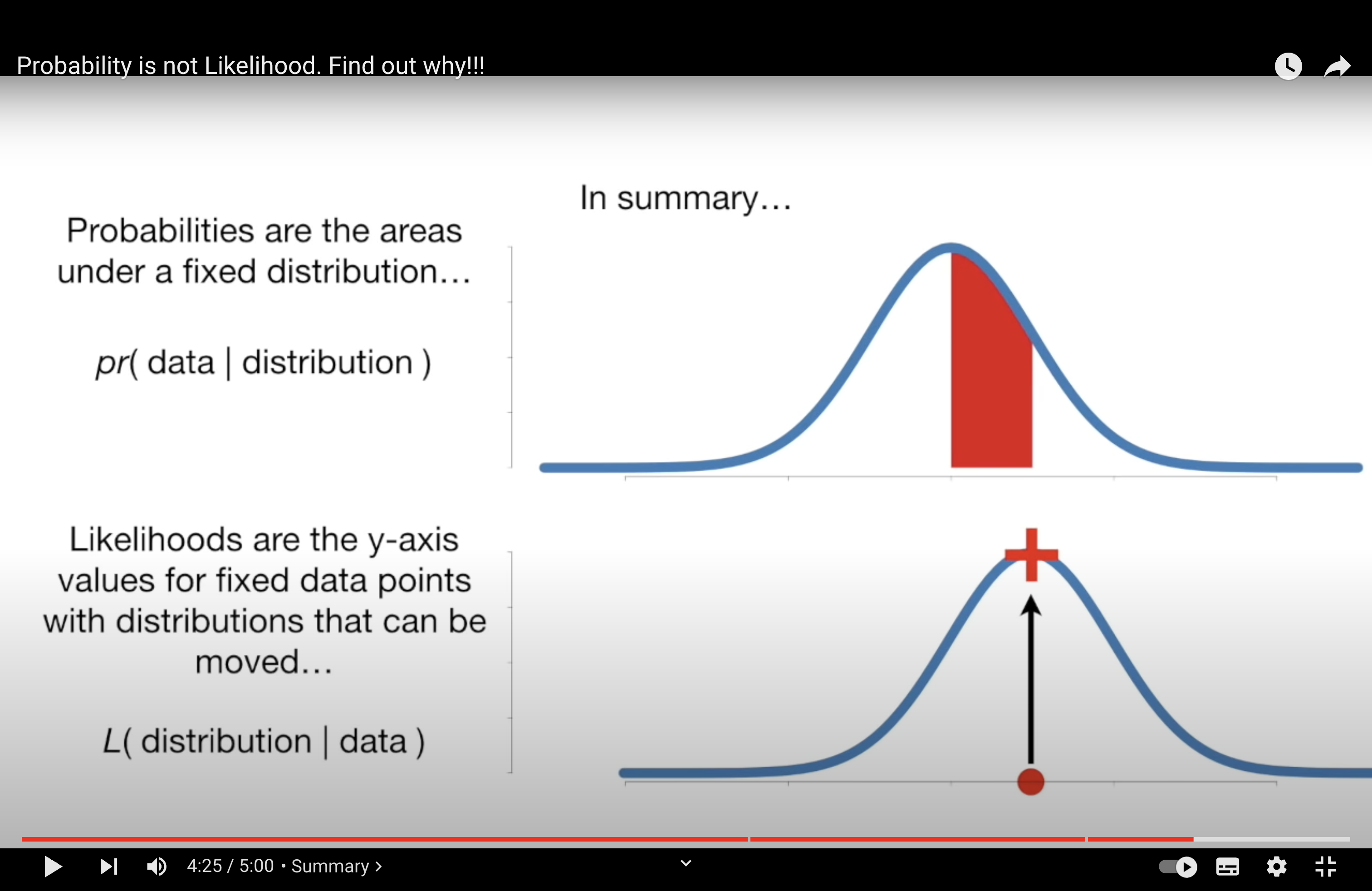
Likelihood and Prob#
Probability is not Likelihood. Find out why!!!