Review 3#
This notes is completed with assistance of ChatGPT
ToC#
Iterative optimization
gradient descent, Newton Raphson
Regularization
PAC, VC dimension
normal equation#
The normal equation is a method used to find the optimal parameters for a linear regression model without resorting to iterative optimization techniques like gradient descent. If you have a design matrix \( X \) (with each row being a training example and each column being a feature) and a vector \( y \) of target values, the normal equation provides a formula to directly compute the optimal weight vector \( \theta \) for the linear regression model.
The formula for the normal equation is:
Where:
\( \theta \) is the vector of model parameters.
\( X \) is the design matrix.
\( y \) is the vector of target values.
\( X^T \) is the transpose of \( X \).
\( (X^T X)^{-1} \) is the inverse of the matrix \( X^T X \).
This equation gives you the parameter values that minimize the cost function for linear regression. However, it’s worth noting that the normal equation can be computationally expensive for very large datasets or when \( X^T X \) is non-invertible (singular). In such cases, iterative methods like gradient descent might be more appropriate.
Newton Raphston#
Question
“Recall that linear regression’s objective can be written as \( L(\theta) = \frac{1}{2} ||X\theta - y||^2 \), where \( X \) is a \( n \times d \) matrix of training instances in rows, \( y \in \mathbb{R}^n \) are the training labels, and \( \theta \in \mathbb{R}^d \) are the parameters to learn by minimising \( L(\theta) \). Show that for any starting \( \theta \in \mathbb{R}^d \), a single step of Newton-Raphson optimisation of \( L(\theta) \) recovers the normal equation exact solution. (Hints for taking vector/matrix-valued derivatives with respect to \( \theta \), for constants matrix \( A \) and vector \( b \). Hint 1: \( \nabla (A\theta + b) = A \). Hint 2: \( \nabla^2(A\theta) = A \). Hint 3: \( \nabla ||f (\theta)||^2 \) = \( 2 \nabla f(\theta)^T f(\theta) \). Where prime ‘ denotes transpose, \( \nabla \) the gradient, and \( \nabla^2 \) the Hessian as in class, here always with respect to \( \theta \)).”
Answer
Alright, let’s correct that and go through the process again.
Given the objective function:
We want to show that a single step of the Newton-Raphson optimization recovers the normal equation solution.
The Newton-Raphson update rule for optimization is:
Step 1: Compute the gradient \( \nabla L(\theta) \).
Using the given hints:
The gradient is:
Step 2: Compute the Hessian \( \nabla^2 L(\theta) \).
Using the hint:
The Hessian is:
Step 3: Plug into the Newton-Raphson update rule.
Notice that if \( \theta_{\text{old}} \) is any arbitrary starting point, then \( \theta_{\text{new}} \) will be the solution of the normal equation:
This shows that a single step of Newton-Raphson optimization recovers the normal equation exact solution.
PAC#
The formula you provided breaks down the excess risk of a learned model \( f_m \) into two components: the estimation error and the approximation error. Let’s dissect the formula and its components:
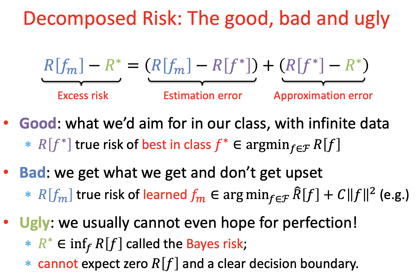
Excess Risk:
This represents the difference in risk (or error) between the model \( f_m \) that we’ve learned from our data and the optimal model with the lowest possible risk \( R^* \). This difference is what we refer to as the “excess risk” of \( f_m \).
Estimation Error:
This is the difference in risk between the model \( f_m \) and the best possible model \( f^* \) from our hypothesis class. The estimation error arises because of the limitations of our learning algorithm and the finite amount of data we have. It captures the error due to the “estimation” process of learning \( f_m \) from data.
Approximation Error:
This represents the difference in risk between the best possible model \( f^* \) from our hypothesis class and the optimal model with the lowest possible risk \( R^* \). The approximation error arises because our hypothesis class might not contain the optimal model. It captures the error due to the “approximation” of the true underlying function by the best function in our hypothesis class.
To summarize:
Excess Risk: The total additional risk our learned model \( f_m \) has compared to the optimal model.
Estimation Error: The error due to the process of learning a model from data.
Approximation Error: The error due to the limitations of our hypothesis class in approximating the true underlying function.
The formula essentially decomposes the excess risk into these two main sources of error, helping us understand where the shortcomings of our learned model come from.
PAC Learning#
What: A framework for the mathematical analysis of machine learning
Goal:
The goal is with high probability, the selected hypothesis will have lower error.
AKA achieve low generalization error with high prob.
AKA we want our model to be approximately correct as much as possible where
approximately correct is up-bounded by the error rate (\(\epsilon\)) and
as much as possible is low-bounded by \(\delta\)
where both \(\epsilon\) and \(\delta\) are very small numbers.
Why not \(\delta = 0\) ?
In real word scenario, we don’t know the data distribution. Hence we need a general framework to set the indications.
Parameters:
\(\epsilon\) gives an upper bound on the error in accuracy with which h approximated (accuracy: \(1 - \epsilon\)) \(\delta\) gives the probability of failure in achieving this accuracy (confidence: \(1 - \delta\))
Tip
In the PAC model, we specify two small parameters, \(\epsilon\) and \(\delta\), and require that with probability at least \(1 - \delta\) a system learn a concept with error at most \(\epsilon\).
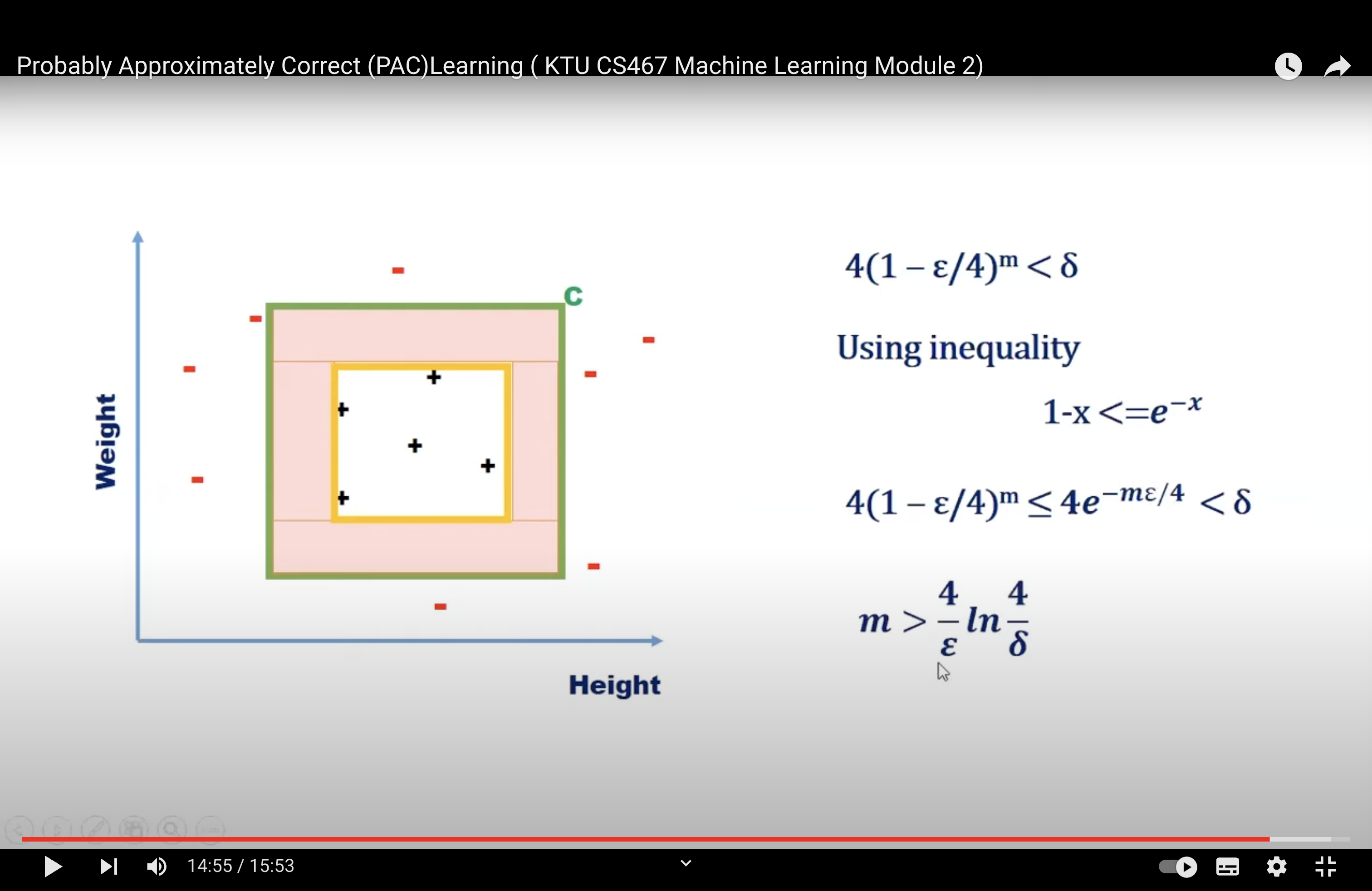
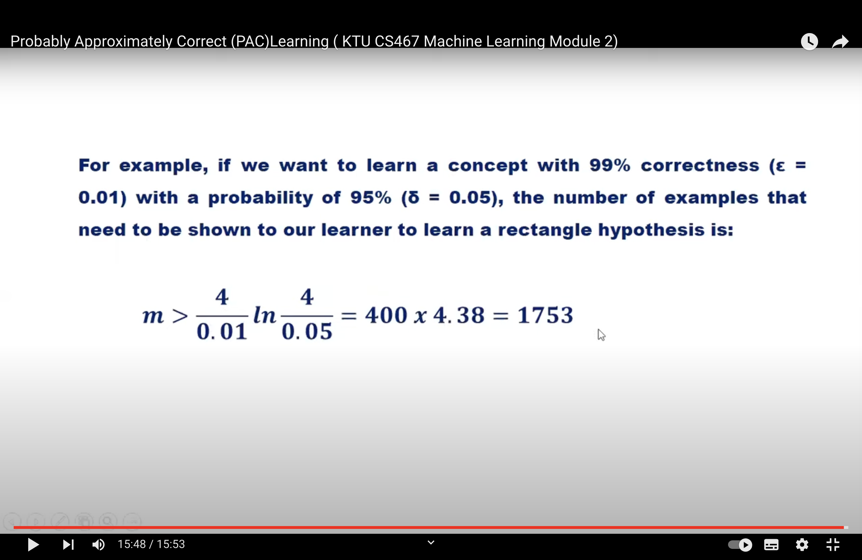
That is if we want to have an accuracy of € and confidence of at least \(1 - \delta\) we have to choose a sample size m such that:
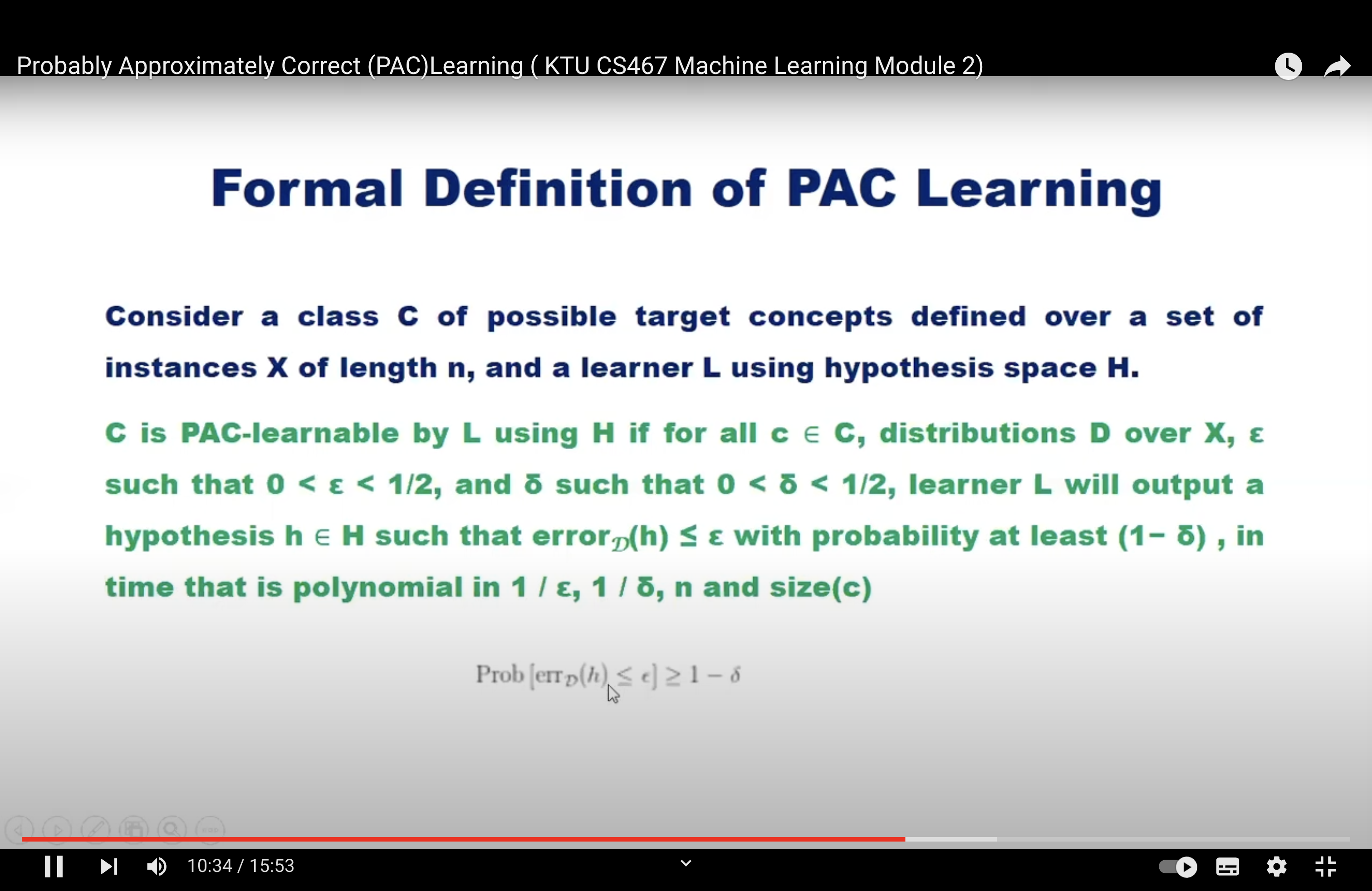
PAC Learnability#
A concept class \( F \) is said to be PAC learnable if there exists a polynomial-time learning algorithm such that for any target concept \( f \) in \( F \), any distribution \( D \) over the input space, and for any \( \epsilon, \delta > 0 \) (where \( \epsilon \) is the approximation error and \( \delta \) is the probability bound), the algorithm will, with probability at least \( 1 - \delta \), output a hypothesis \( h \) whose error is at most \( \epsilon \), provided it is given a number of samples \( m \) that is polynomial in \( \frac{1}{\epsilon} \) and \( \frac{1}{\delta} \).
The notation \( m = \mathcal{O}(\text{poly}(\frac{1}{\epsilon}, \frac{1}{\delta})) \) means that the sample complexity \( m \) is bounded by a polynomial function of \( \frac{1}{\epsilon} \) and \( \frac{1}{\delta} \).
However, the statement “if \( m = 0 \)” is confusing in this context. If \( m \) is 0, it means no samples are required, which doesn’t make sense in the PAC learning framework. It’s possible there’s a misunderstanding or miscommunication about the notation or concept. If you have a specific question or context about PAC learnability, please provide more details.
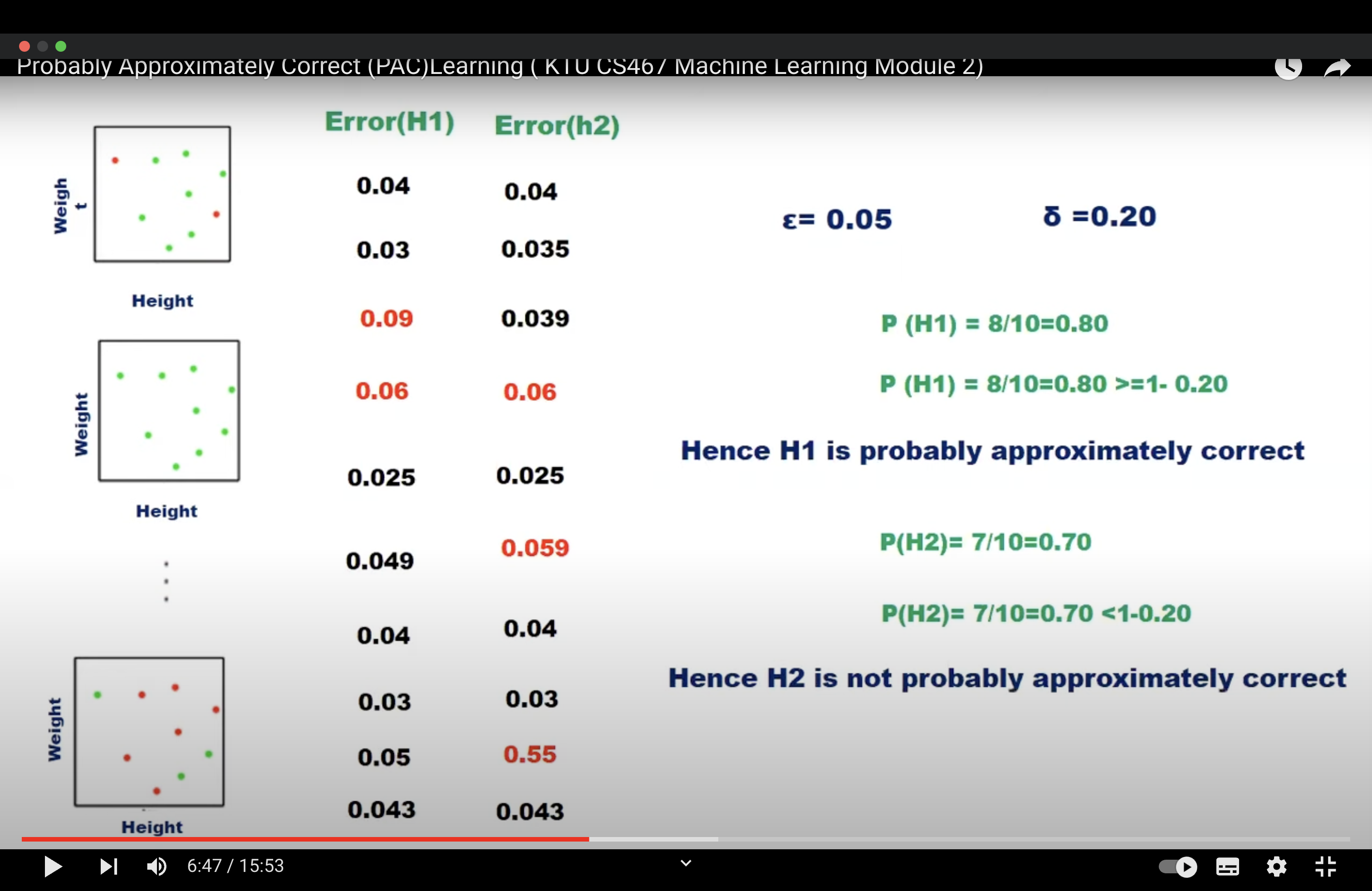
Example
Certainly! Let’s break down the concept of PAC (Probably Approximately Correct) learning into simpler terms.
Imagine you’re trying to teach a robot to recognize cats. You show the robot a bunch of pictures, some of cats and some of other things. After this training, you want the robot to correctly identify new pictures of cats that it hasn’t seen before.
Now, let’s relate this to the PAC learning framework:
Concept Class \( \mathcal{F} \): This is like the set of all possible “rules” or “methods” the robot could use to identify cats. Each rule or method is a “concept”.
Target Concept \( f \) in \( \mathcal{F} \): This is the “correct rule” for identifying cats. We assume there’s a right way to do it, even if we don’t know what it is.
Distribution \( \mathcal{D} \) over the input space: This is like saying that some pictures are more likely to be shown to the robot than others. For example, maybe close-up pictures of cats are more common than distant ones.
\( \epsilon \) (Approximation Error): This is how much error we’re willing to tolerate. If \( \epsilon \) is 0.05, then we’re okay if the robot gets 5% of new cat pictures wrong.
\( \delta \) (Probability Bound): This is our confidence level. If \( \delta \) is 0.01, then we want to be 99% sure that the robot’s error is at most \( \epsilon \).
PAC Learnable: A set of rules (or concepts) is PAC learnable if there’s a way (an algorithm) to teach the robot so that, after seeing a certain number of pictures, it can recognize new cat pictures with an error rate of at most \( \epsilon \) and we’re \( 1-\delta \) confident in this.
Polynomial-time learning algorithm: This means that the time it takes for the robot to learn doesn’t grow too fast as we show it more pictures or demand higher accuracy.
Sample Complexity \( m \): This is the number of pictures we need to show the robot for it to learn well. If our set of rules is PAC learnable, then the number of pictures (samples) we need to show the robot is reasonable (i.e., it’s not an astronomically large number).
The notation \( m = \mathcal{O}(\text{poly}(1/\epsilon, 1/\delta)) \) is a mathematical way of saying that the number of pictures we need to show the robot grows in a “polynomial” way based on how accurate we want it to be (\( \epsilon \)) and how confident we want to be in its accuracy (\( \delta \)). In simpler terms, it means that if we want the robot to be more accurate or more confident, we might need to show it more pictures, but not an unreasonable amount more.
In essence, PAC learning is a framework that helps us understand when and how we can teach algorithms to generalize well from training data to new, unseen data.
The exact number of pictures (or samples) you need to show depends on several factors:
The Complexity of the Hypothesis Class: If the set of rules (concepts) the robot can use to identify cats is very complex, you might need more samples to ensure you’ve covered enough cases for the robot to generalize well.
Desired Accuracy (\( \epsilon \)): If you want the robot to be very accurate (low \( \epsilon \)), you’ll need more samples. For instance, if you want the robot to be 99% accurate, you’ll need more pictures than if you’re okay with it being 90% accurate.
Confidence Level (\( \delta \)): If you want to be very confident in the robot’s accuracy, you’ll need more samples. For example, if you want to be 99.9% sure of the robot’s performance, you’ll need more pictures than if you’re okay with being 95% sure.
Distribution of the Data (\( \mathcal{D} \)): If the pictures you have are very diverse and cover a wide range of cat scenarios (e.g., different breeds, lighting conditions, angles), you might need fewer samples than if your pictures are very similar.
The notation \( m = \mathcal{O}(\text{poly}(1/\epsilon, 1/\delta)) \) gives a general idea of how the number of samples grows with \( \epsilon \) and \( \delta \), but it doesn’t give an exact number. It says that the number of samples grows polynomially with \( 1/\epsilon \) and \( 1/\delta \). In practice, the exact number also depends on the specific learning problem and the algorithm used.
For a more concrete answer in the context of PAC learning, one would typically derive a bound on the sample complexity based on the VC dimension of the hypothesis class and the desired \( \epsilon \) and \( \delta \). This bound would give an upper limit on the number of samples required to achieve the desired accuracy and confidence. However, in real-world applications, it’s common to use empirical methods, like cross-validation, to determine an appropriate sample size or to check the performance of a model.
PAC Cont.#
The equations you’ve provided are related to the PAC (Probably Approximately Correct) learning framework and the generalization bounds of learning algorithms. These bounds provide a theoretical guarantee on the performance of a learning algorithm on unseen data based on its performance on the training data. Let’s break down the concepts:
True Risk of One Function:
This equation provides a bound on the true risk (or error) \( R[f] \) of a function \( f \) in terms of its empirical risk \( \hat{R}[f] \) (i.e., its error on the training data) and the number of training samples \( m \). The term \( \sqrt{\frac{\log(1/\delta)}{2m}} \) is a confidence interval that ensures the bound holds with high probability at least \( 1-\delta \).
How did we obtain \(\sqrt{\frac{\log(1/\delta)}{2m}}\)
The term \( \sqrt{\frac{\log(1/\delta)}{2m}} \) is a common term that arises in generalization bounds in the context of PAC learning, especially when using concentration inequalities like Hoeffding’s inequality.
Let’s derive this term using Hoeffding’s inequality:
Hoeffding’s Inequality: Given independent random variables \( X_1, X_2, \ldots, X_m \) that are bounded such that \( a_i \leq X_i \leq b_i \) for all \( i \), let \( S_m = \sum_{i=1}^{m} X_i \). Then, for any \( t > 0 \):
Now, consider the case of binary classification where each \( X_i \) represents the error of a hypothesis on a single example, so \( X_i \in \{0, 1\} \). This means \( a_i = 0 \) and \( b_i = 1 \) for all \( i \). The bound becomes:
Setting the right-hand side to \( \delta \) (our desired confidence level) and solving for \( t \) gives:
This \( t \) is the amount by which the empirical mean (observed average error on the training set) can deviate from the expected mean (true error) with high probability.
In the context of PAC learning, this term provides a bound on the difference between the empirical risk (error on the training set) and the true risk (expected error on the entire distribution) of a hypothesis. The bound ensures that the empirical risk is a good approximation of the true risk with high probability.
True Risk of a Family:
This equation bounds the true risk of the empirical risk minimizer \( \hat{f}_m \) (the function that has the lowest empirical risk in the hypothesis class). The term \( \sup_{f \in \mathcal{F}} |\hat{R}[f] - R[f]| \) represents the maximum difference between empirical and true risk over all functions in the hypothesis class \( \mathcal{F} \). This difference is often referred to as the “uniform divergence.” The term \( R[f^*] \) is the risk of the best possible function in the hypothesis class.
Why is it 2sup
The term \( 2 \sup_{f \in \mathcal{F}} |\hat{R}[f] - R[f]| \) that you’re referring to is related to the generalization bound in the context of PAC learning. Let’s break it down:
The term \( \sup_{f \in \mathcal{F}} |\hat{R}[f] - R[f]| \) represents the maximum difference between the empirical risk (risk on the training set) and the true risk (expected risk on the entire distribution) over all functions in the hypothesis class \( \mathcal{F} \). This difference is often referred to as the “uniform divergence” or “uniform deviation.”
The factor of 2 in front of the supremum is a result of symmetrization arguments used in the derivation of generalization bounds. Here’s a high-level idea:
When deriving generalization bounds, one common technique is to introduce a set of independent and identically distributed (i.i.d.) “ghost” or “shadow” samples. These are hypothetical samples that come from the same distribution as the training data but are not actually observed. By comparing the performance of hypotheses on the actual training data and the ghost samples, one can derive bounds on the generalization error.
The introduction of ghost samples effectively doubles the deviation between the empirical risk and the true risk, leading to the factor of 2 in the bound. This symmetrization technique simplifies the analysis and is a common step in the derivation of generalization bounds in statistical learning theory.
In essence, the factor of 2 accounts for the worst-case scenario in which the empirical risk underestimates the true risk by the maximum possible amount, and it ensures that the derived bound is valid with high probability across all functions in the hypothesis class.
True Risk of Finite Families:
For a finite hypothesis class \( \mathcal{F} \), this equation provides a bound on the true risk of the empirical risk minimizer \( \hat{f}_m \). The term \( \sqrt{\frac{\log |\mathcal{F}| + \log(1/\delta)}{m}} \) is a confidence interval that accounts for the size of the hypothesis class and ensures the bound holds with high probability.
The derivation of these bounds involves a combination of probability theory (especially concentration inequalities like Hoeffding’s inequality or the union bound) and combinatorial arguments related to the complexity of the hypothesis class (like the VC dimension). The goal of these bounds is to provide theoretical guarantees on the performance of learning algorithms, helping to understand their generalization capabilities.
How is \(\sqrt{\frac{\log |F| + \log(1/\delta)}{m}}\) calculated
This term is a generalization bound often associated with the true risk of finite hypothesis classes in the Probably Approximately Correct (PAC) learning framework. This bound is derived using concentration inequalities, especially the union bound and Hoeffding’s inequality. Let’s break down its derivation:
Hoeffding’s Inequality for a Single Hypothesis: For a single hypothesis \( f \) from a finite hypothesis class \( F \), the difference between its empirical risk \( \hat{R}[f] \) (observed on the training set) and its true risk \( R[f] \) (over the entire distribution) can be bounded using Hoeffding’s inequality:
This says that the true risk of \( f \) exceeds its empirical risk by more than \( \sqrt{\frac{\log(2/\delta)}{2m}} \) with probability less than \( \delta \).
Union Bound for Multiple Hypotheses: Since \( F \) is a finite hypothesis class, we can apply the union bound to account for all hypotheses in \( F \). The union bound states that the probability of any one of several events occurring is at most the sum of their individual probabilities.
Let’s say we want the above bound to hold for all hypotheses in \( F \) simultaneously with a confidence of at least \( 1-\delta \). Using the union bound:
Where \( \delta' \) is the probability for a single hypothesis. If we set \( |F| \cdot \delta' = \delta \), then \( \delta' = \frac{\delta}{|F|} \).
Combining the Bounds: Substituting \( \delta' \) into the bound from Hoeffding’s inequality:
This bound ensures that the true risk of every hypothesis in \( F \) is close to its empirical risk with high probability.
Simplifying: For clarity and simplicity, the bound is often written as:
This is the generalization bound for finite hypothesis classes in the PAC framework, and it provides a theoretical guarantee on the performance of a learning algorithm on unseen data based on its performance on the training data.
VC dimension#
Def#
Vapnik-Chervonenkis (VC) Dimension The maximum number of points that can be shattered by H is called the Vapnik-Chervonenkis dimension of H. VC dimension is one measure that characterizes the expressive power or capacity of a hypothesis class
The VC (Vapnik-Chervonenkis) dimension is a fundamental concept in statistical learning theory. It provides a measure of the capacity or complexity of a hypothesis class. Specifically, the VC dimension gives an upper bound on the number of training samples that a hypothesis class can shatter, which in turn provides insights into the generalization ability of a learning algorithm.
Here’s a more detailed breakdown:
Shattering: A hypothesis class \( H \) is said to “shatter” a set of points if, for every possible labeling of those points (binary labels, typically 0 or 1), there exists some hypothesis in \( H \) that perfectly separates the points according to that labeling.
VC Dimension: The VC dimension of a hypothesis class \( H \) is the largest number of points that \( H \) can shatter. If \( H \) can shatter an arbitrarily large number of points, then its VC dimension is said to be infinite.
Implications for Learning:
A higher VC dimension indicates that the hypothesis class is more complex and can represent a wider variety of functions.
However, a higher VC dimension also means that the hypothesis class can easily overfit to the training data. This is because a more complex hypothesis class can fit the training data in many ways, including fitting to the noise in the data.
The VC dimension plays a crucial role in deriving generalization bounds in machine learning. Specifically, it helps in determining how well a learning algorithm will perform on unseen data, given its performance on the training data.
Examples:
For a hypothesis class of linear classifiers in 2D (lines in the plane), the VC dimension is 3. This is because any 3 non-collinear points can be shattered by lines in the plane, but 4 general points cannot be.
For a hypothesis class of linear classifiers in \( d \)-dimensions (hyperplanes), the VC dimension is \( d + 1 \).
Relationship with PAC Learning: In the PAC (Probably Approximately Correct) learning framework, the VC dimension helps determine the number of samples required to learn a concept within a certain error bound. Specifically, if the VC dimension is finite, then the sample complexity for PAC learning is polynomial in terms of the VC dimension, the inverse of the desired error \( \epsilon \), and the inverse of the confidence \( \delta \).
The VC dimension provides a bridge between the empirical performance of a learning algorithm (its performance on the training set) and its expected performance on unseen data, making it a foundational concept in understanding the generalization capabilities of learning algorithms.
Tip
N data points can be classified in \(2^N\) ways
what is VC dimension why do we need it?
The VC (Vapnik-Chervonenkis) dimension is a measure of the capacity or complexity of a hypothesis class in machine learning. It quantifies the expressive power of a class of functions by determining the largest set of points that can be shattered (i.e., classified in all possible ways) by that class. A higher VC dimension indicates that the hypothesis class can represent more complex functions.
Example#
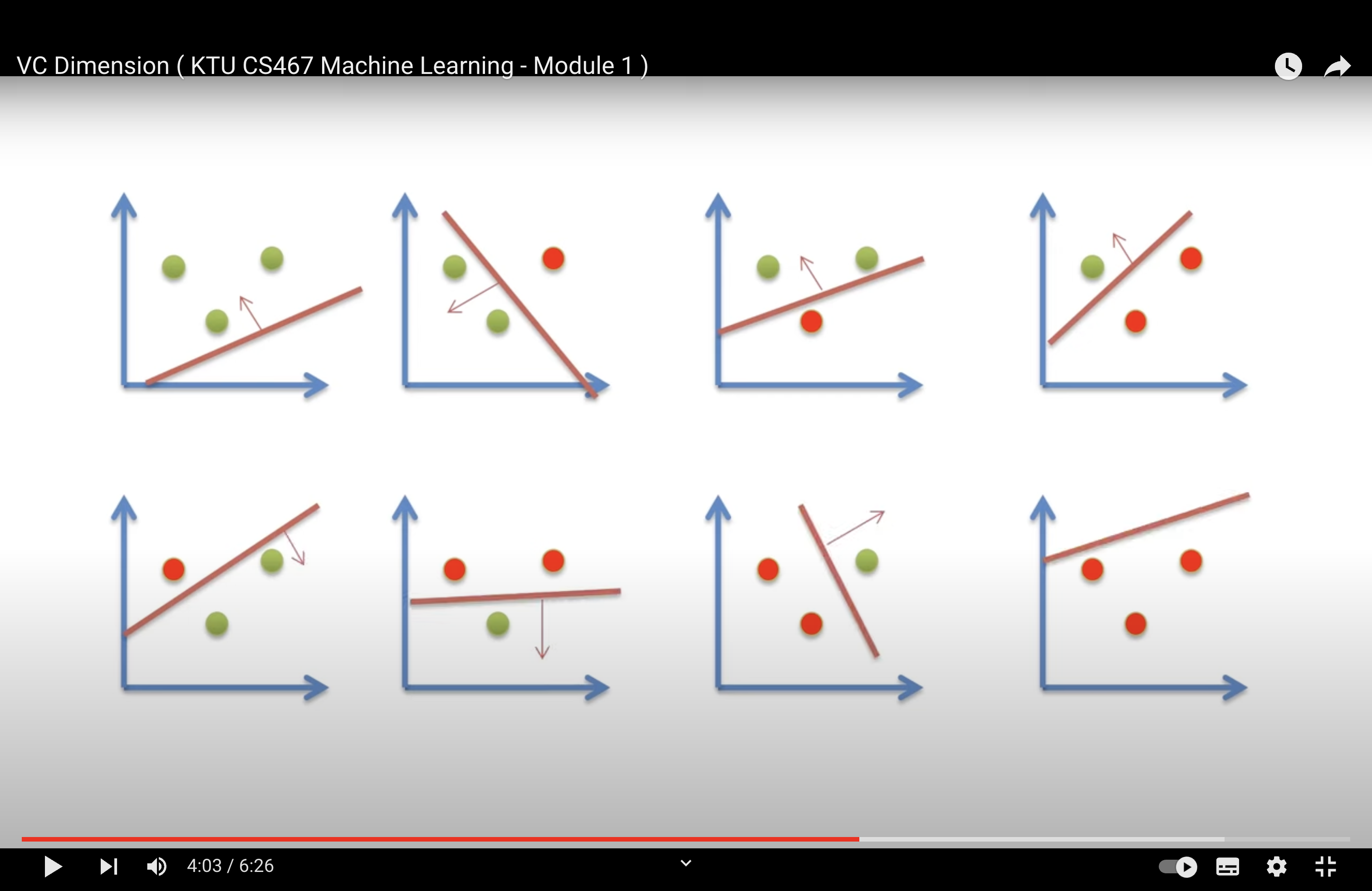
Shattering A set of N points is said to be shattered by a hypothesis space H, if there are hypothesis(h) in H that separates positive examples from the negative examples in all of the 2N possible ways.
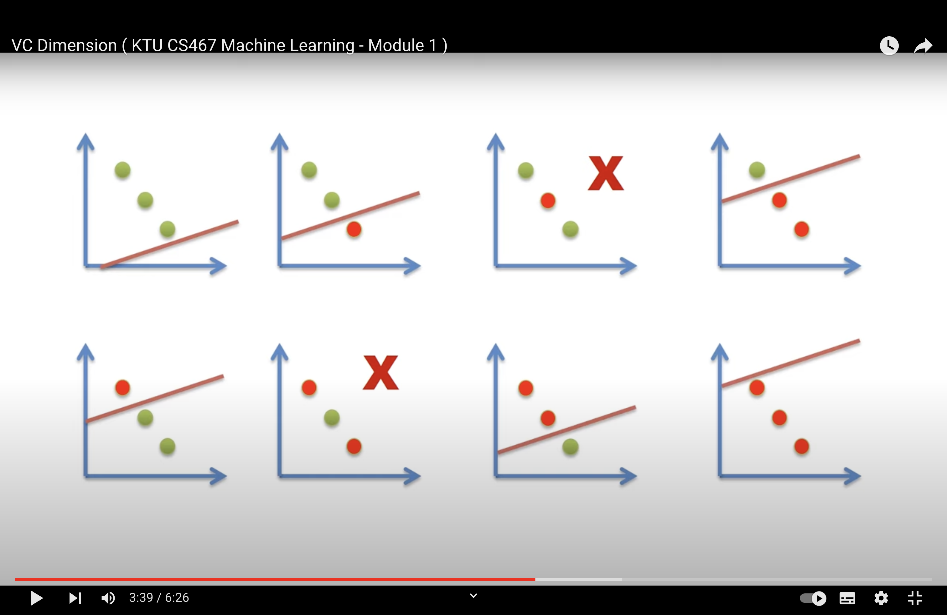
It may not be able to shatter every possible set of three points in 2 dimensions.
It is enough to find one set of three points that can be shattered.
We can’t find a set of 4 points that can be shattered by a single straight line in 2D.
Tip
Hence, Maximum number of points in R2 that be shattered by straight line is 3
Tip
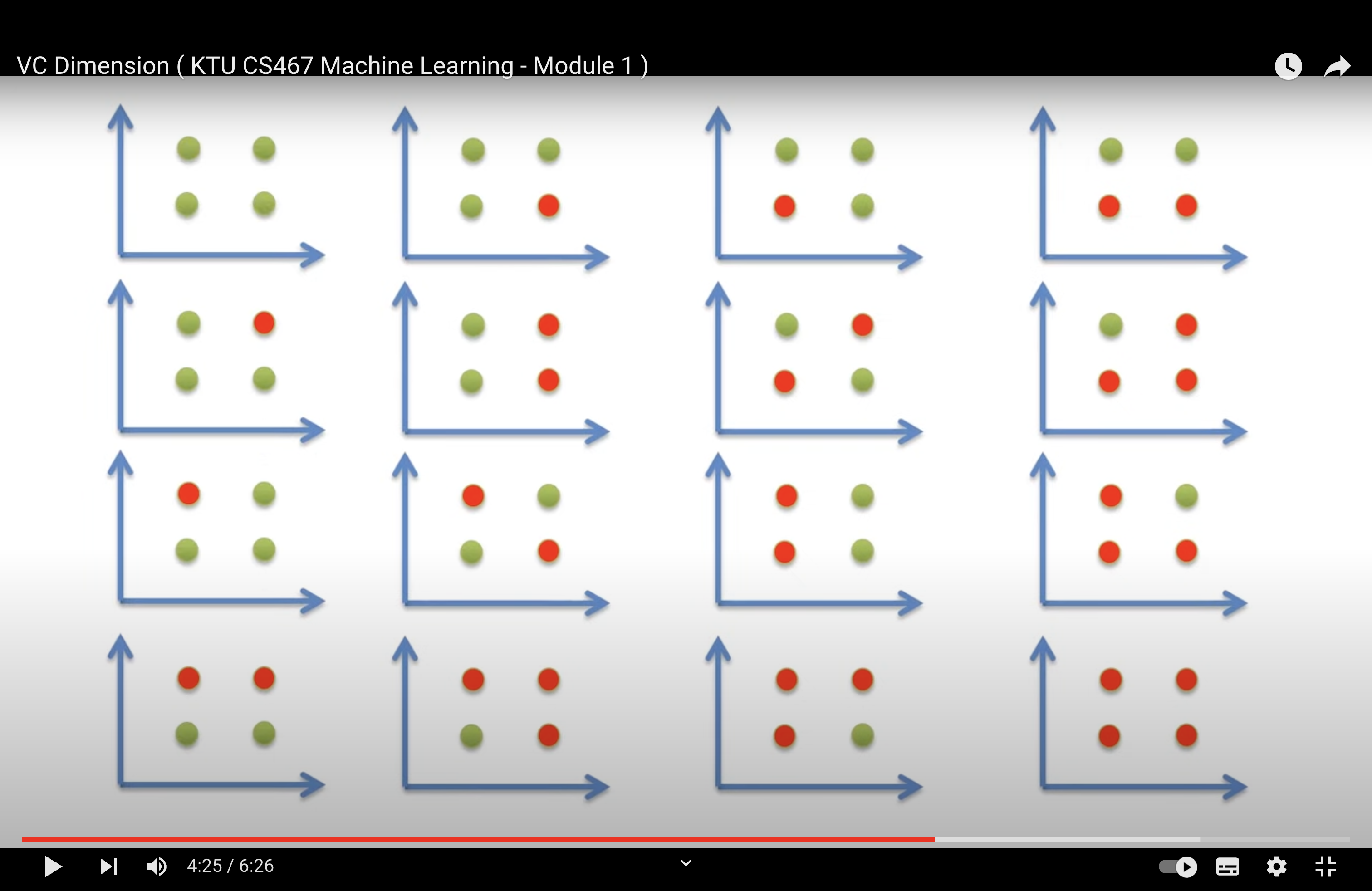
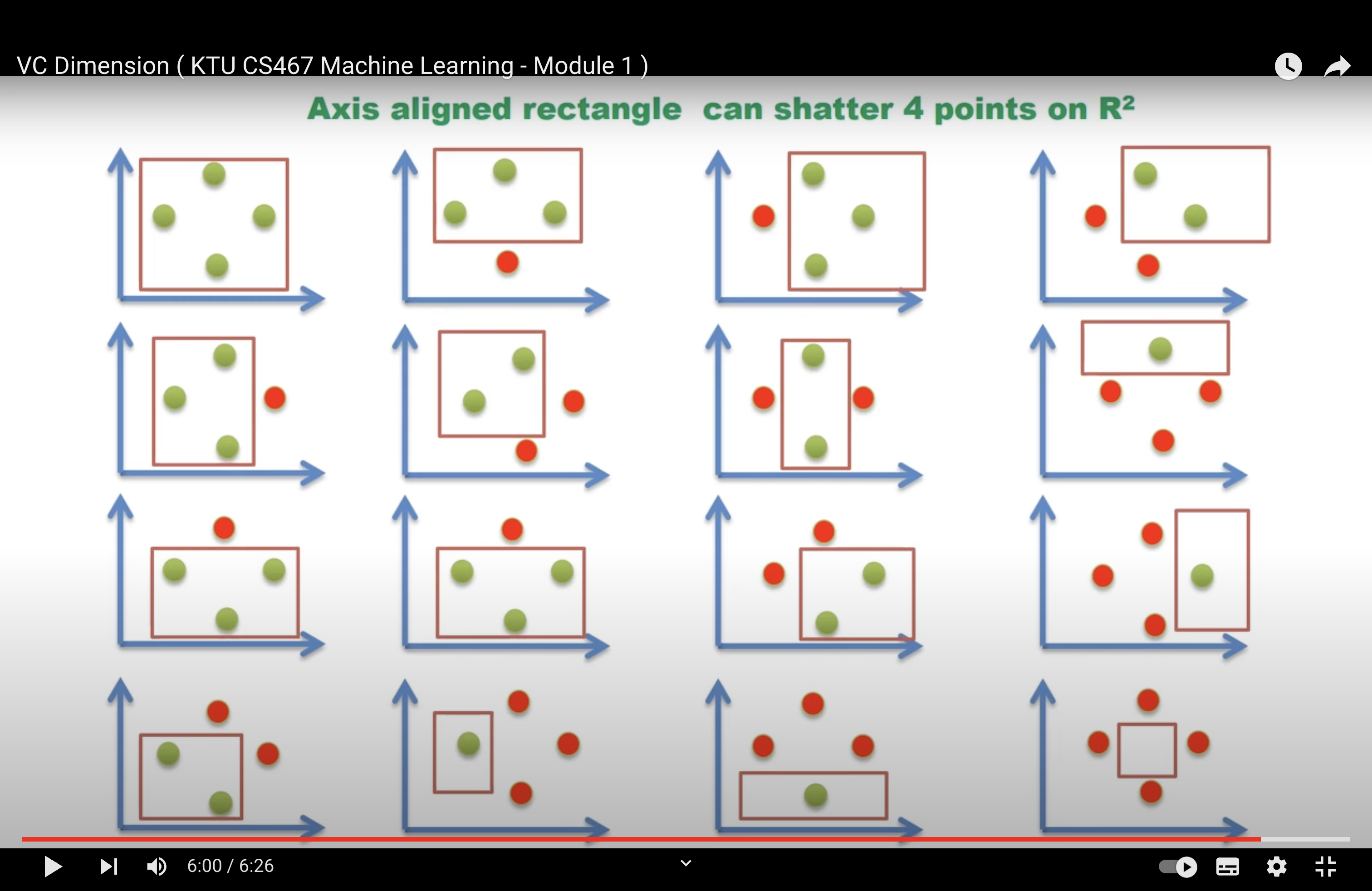
VCD (Axis Aligned Rectangle in R2)= 4
AKA Maximum number of points in R2 that be shattered by a square is 4
Addtional Resource#
PCA#
The mathematical justification of why the eigenvectors of the covariance matrix point to the directions of maximum variance.
Given:
A data matrix \( X \) of size \( n \times m \) where \( n \) is the number of observations and \( m \) is the number of features. The data is mean-centered (i.e., the mean of each feature is zero).
The covariance matrix \( C \) is given by:
We want to find the direction \( w \) (a unit vector) that maximizes the variance of the projected data.
The variance \( V \) of the data projected onto \( w \) is given by:
Under the constraint that \( w \) is a unit vector, the above expression is maximized when \( w \) is the eigenvector of \( C \) corresponding to its largest eigenvalue.
Proof:#
To maximize \( V \) under the constraint \( ||w|| = 1 \) (where \( ||\cdot|| \) denotes the Euclidean norm), we can use the method of Lagrange multipliers.
Consider the Lagrangian:
Taking the gradient with respect to \( w \) and setting it to zero, we get:
This is the eigenvalue equation! It says that \( w \) is an eigenvector of \( C \) and \( \lambda \) is the corresponding eigenvalue.
To maximize the variance \( V = w^T C w \), we need \( w \) to be the eigenvector corresponding to the largest eigenvalue of \( C \).
Conclusion:#
The direction \( w \) that maximizes the variance of the projected data is the eigenvector of the covariance matrix \( C \) corresponding to its largest eigenvalue. Similarly, subsequent principal components (orthogonal to the first) align with eigenvectors corresponding to decreasing eigenvalues.