Review 2#
This notes is completed with assistance of ChatGPT
ToC#
Kernel Trick
common kernels
prove valid kernel
Discriminative Neural Networks Models
Perceptron
Feedforward Neural Networks
Convolutional Neural Networks
Recurrent Neural Networks
Attention
SVM vs NN#
Question
What is the difference between Feedforward Neural Networks and SVM considering their approaches in dealing with non-linearly separable data?
Answer
Feedforward Neural Networks (FNNs) and Support Vector Machines (SVMs) both handle non-linearly separable data, but they approach the problem differently. FNNs, especially when equipped with non-linear activation functions, learn hierarchical representations of data by transforming input through multiple layers, allowing them to approximate any function, including non-linear boundaries. SVMs, on the other hand, utilize the kernel trick to map the input data into a higher-dimensional space where it becomes linearly separable. Instead of learning representations like FNNs, SVMs focus on finding the optimal hyperplane that maximally separates the classes in this transformed space.
Question
What are the advantage and disadvantage of manual feature engineering and automatic data transformation in Neural Network Models?
Answer
The advantages and disadvantages of manual feature engineering and automatic data transformation in neural network models:
Aspect |
Manual Feature Engineering |
Automatic Data Transformation in Neural Network Models |
|---|---|---|
Advantages |
||
Domain Knowledge Application |
✅ Uses domain expertise to create meaningful features. |
❌ Lacks domain-specific insights. |
Model Interpretability |
✅ Leads to transparent and interpretable models. |
❌ Often results in “black box” models. |
Efficiency |
✅ Simpler models might suffice. |
❌ Requires complex models and more computational resources. |
Adaptability |
❌ Might not generalize across tasks. |
✅ Adaptable to various tasks without manual intervention. |
End-to-end Learning |
❌ Typically not end-to-end. |
✅ Allows optimization from raw data to output. |
Reduced Human Bias |
❌ Risk of introducing biases based on intuitions. |
✅ Reduces human biases in feature creation. |
Disadvantages |
||
Time Consumption |
✅ Requires significant time and effort. |
❌ Faster adaptation to new data/tasks. |
Risk of Overfitting |
✅ Possible if features don’t generalize well. |
❌ Can overfit if not regularized or if data is limited. |
Scalability |
❌ Needs repeated efforts for new tasks/data. |
✅ Scales better to different tasks without manual changes. |
Note: The “✅” and “❌” symbols indicate whether the mentioned aspect is an advantage or disadvantage, respectively, for each method.
Partial Derivative of Loss Function#
Question
Given the following neural network for binary classification, if we use binary cross entropy as loss function, compute the partial derivative of loss function L with respect to vij (written as a formula that only contains xi, uj, wj, z and y, where y is the correct label of data. Assume we use sigmoid activation function everywhere, which are shown as f in the figure below.)
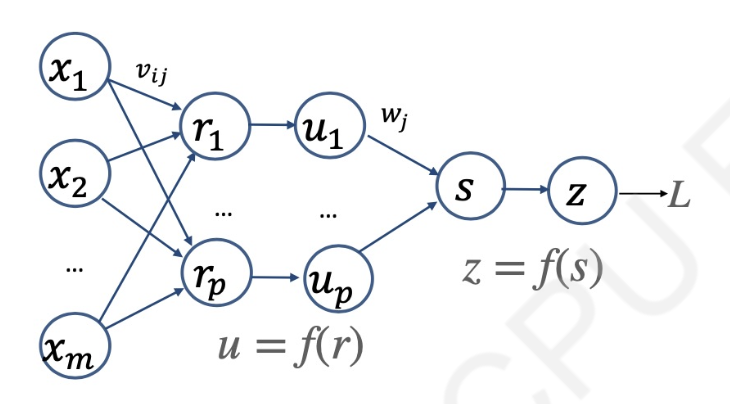
Answer
Alright, let’s compute the derivative of the binary cross entropy loss with respect to \( v_{ij} \).
Given: Loss function \( L \) for binary classification with binary cross entropy:
Where:
and
Given that \( f \) is the sigmoid function:
The derivative \( f'(x) \) is:
From the given neural network:
or
where \( r_j \) is the net input to neuron \( j \) in the hidden layer.
Let’s compute the chain of derivatives:
Derivative of \( L \) with respect to \( z \):
Derivative of \( z \) with respect to \( s \):
Derivative of \( s \) with respect to \( u_j \):
Derivative of \( u_j \) with respect to \( r_j \):
Derivative of \( r_j \) with respect to \( v_{ij} \):
Using the chain rule, the partial derivative of \( L \) with respect to \( v_{ij} \) is:
Substitute in the computed derivatives:
After simplifying:
And this is the partial derivative of the loss function \( L \) with respect to \( v_{ij} \).
Derivative of Sigmoid Function#
Given:
To find \( f'(x) \), differentiate with respect to \( x \):
Notice:
So:
Replacing \( e^{-x} \) in the derivative expression:
So, the derivative of the sigmoid function is:
Tip
Use the quotient rule of differentiation: If you have a function in the form \( \frac{u(x)}{v(x)} \), then its derivative is:
CNN#
Pooling#
Calculations#
(a)Size of Output Map
Where:
\( O \) is the output size.
\( W \) is the width (or height) of the input.
\( K \) is the kernel (or filter) size.
\( P \) is the padding.
\( S \) is the stride.
(b) Number of parameters in each layer:
Parameters = \( K × K × C_{in} × C_{out} \)
\( K \) is the kernel size.
\( C_{in} \) is the number of input channels.
\( C_{out} \) is the number of output channels (or filters). eg. input: 64 * 64 * 64 * 3 -> 3 is the number of input channels;
output channels = # of filters.
Pooling: No learnable parameters in max-pooling layer.
Fully Connected:
n * m (no bias)
(n + 1) * m (with bias)
(c) To keep the same size of the receptive field of conv2 with fewer parameters:
Use 1x1 Convolution (a.k.a Network in Network): Applying 1x1 convolutions can help reduce the depth (number of channels) before applying the 9x9 convolution. For example, using a 1x1 convolution to reduce the channels to 32, and then applying a 9x9 convolution.
Use Dilated Convolution: Instead of the regular convolution, dilated (or atrous) convolution can be used with a smaller kernel size but with increased dilation rate to achieve the same receptive field.
Factorized Convolution: Decompose the 9x9 convolution into two separate convolutions: one 9x1 convolution followed by a 1x9 convolution.
Note: Each of the above methods reduces the number of parameters while maintaining the same receptive field, but the exact effects on performance and the number of parameters saved will vary.