Additional Notes - More on Bayesian#
More on Bayesian#
This note is completed with the assistance of ChatGPT
Useful Resources#
Bayesian Regression and Inference Youtube Series
Sum Rule, Product Rule, Joint & Marginal Probability - CLEARLY EXPLAINED with EXAMPLES!
Posterior Predictive Distribution - Proper Bayesian Treatment!🌟🌟🌟
Probabilistic Programming - FOUNDATIONS & COMPREHENSIVE REVIEW!
Joint Distributions#
Why Bayesian Approaches Often Require Working with Joint Distributions:
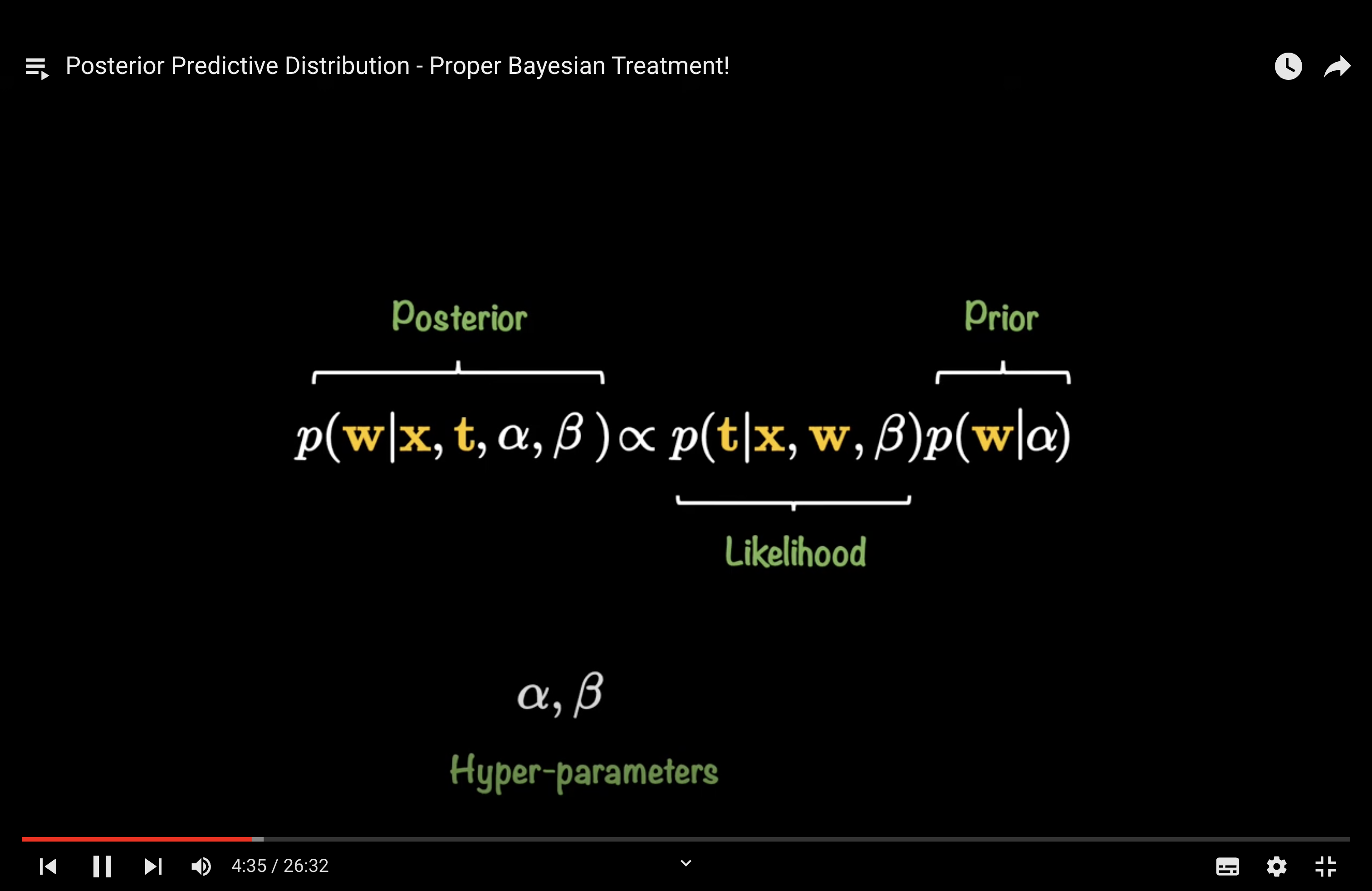
Bayes’ Theorem: The foundation of Bayesian inference is Bayes’ theorem, which relates the joint distribution and the conditional distributions of the variables involved. Specifically, it states:
\[ P(A|B) = \frac{P(B|A) \times P(A)}{P(B)} \]Here, \( P(A|B) \) is the posterior, \( P(B|A) \) is the likelihood, \( P(A) \) is the prior, and \( P(B) \) is the evidence (or marginal likelihood). The evidence is often computed by summing or integrating over the joint distribution of \( A \) and \( B \).
Updating Beliefs: Bayesian approaches are all about updating prior beliefs with new data to get a posterior belief. This updating process inherently involves working with the joint distribution of the data and the parameters.
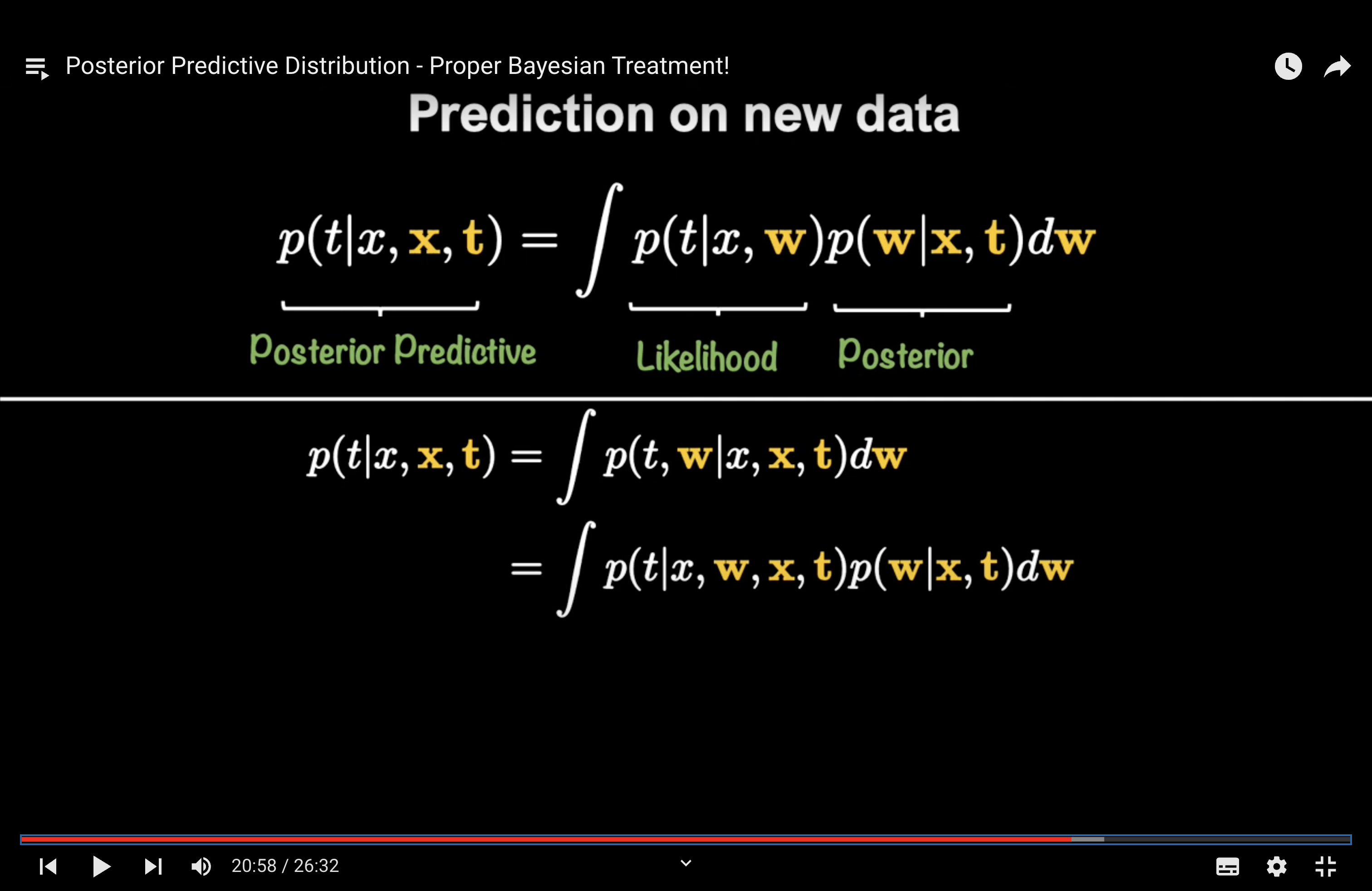
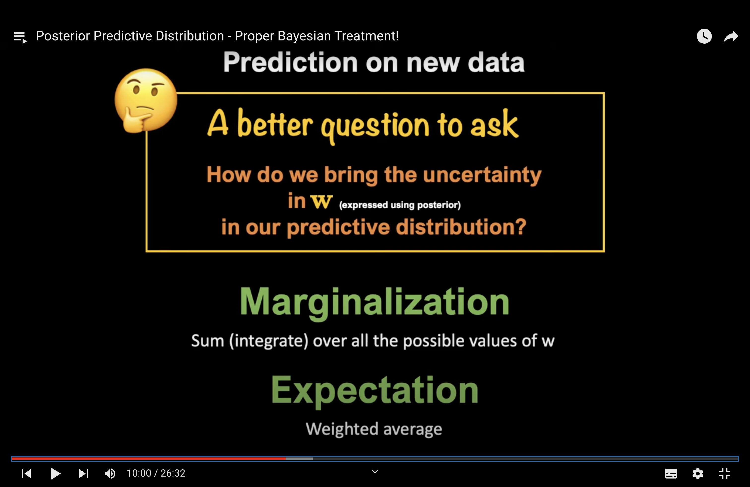
Predictive Distributions: To make predictions in a Bayesian framework, we often need to integrate out the parameters over their joint distribution with the data.
Why Choosing Appropriate Priors is Crucial in Bayesian Modeling:
Influence on the Posterior: The prior represents our belief about a parameter before observing any data. If we have a strong prior belief (informative prior), it can significantly influence the posterior, especially if the amount of data is small. Conversely, if we have little prior knowledge, we might choose a non-informative or weak prior, letting the data play a more significant role in shaping the posterior.
Regularization: Priors can act as regularizers. For instance, a prior that favors smaller values of a parameter can prevent overfitting in a model, similar to L1 or L2 regularization in non-Bayesian contexts.
Incorporating Expert Knowledge: One of the strengths of Bayesian modeling is the ability to incorporate expert knowledge or beliefs into the model through the prior. This can be especially valuable in domains where data is scarce or expensive to obtain.
Model Identifiability: In some cases, without an appropriate prior, a model might be non-identifiable, meaning there could be multiple parameter values that explain the data equally well. A prior can help in pinning down a unique or more plausible solution.
Computational Stability: Priors can also aid in the computational stability of Bayesian inference algorithms, especially in high-dimensional parameter spaces.
In summary, Bayesian approaches inherently involve the manipulation and computation with joint distributions, as they provide a comprehensive view of the relationships between variables and are essential for updating beliefs and making predictions. Priors, on the other hand, are a defining feature of Bayesian modeling, allowing for the incorporation of prior beliefs and playing a crucial role in determining the behavior and properties of the resulting posterior distributions.
Prior and Posterior#
Updating prior beliefs is at the heart of Bayesian inference. The process involves using Bayes’ theorem to combine our prior beliefs (prior distribution) with new evidence (data) to obtain an updated belief (posterior distribution). Here’s a step-by-step breakdown:
Prior represents?
Our beliefs about the parameter(s) P(θ) before observing any data.
Start with a Prior Distribution:
The prior distribution, denoted \( P(\theta) \), represents our beliefs about the parameter(s) \( \theta \) before observing any data. This can be based on previous studies, expert opinion, or other sources of information.
Observe Data and Compute the Likelihood:
The likelihood, denoted \( P(D|\theta) \), tells us how probable our observed data \( D \) is, given different values of the parameter(s) \( \theta \). It quantifies how well different parameter values explain the observed data.
Apply Bayes’ Theorem to Compute the Posterior Distribution:
The posterior distribution, denoted \( P(\theta|D) \), represents our updated belief about the parameter(s) \( \theta \) after observing the data \( D \). It’s computed using Bayes’ theorem:
Here:
\( P(\theta|D) \) is the posterior.
\( P(D|\theta) \) is the likelihood.
\( P(\theta) \) is the prior.
\( P(D) \) is the evidence or marginal likelihood. It’s a normalizing constant ensuring that the posterior distribution integrates (or sums) to 1. It’s computed by integrating (or summing) the numerator over all possible values of \( \theta \):
(For discrete parameters, the integral becomes a sum.)
Interpret the Posterior Distribution:
The posterior distribution combines the information from the prior and the data. If the data are strong and informative, the posterior will be more influenced by the likelihood. If the data are weak or scarce, the prior will play a more significant role in shaping the posterior.
The mode of the posterior distribution gives the Maximum A Posteriori (MAP) estimate of the parameter(s). If you’re interested in point estimates, the MAP is a common choice in Bayesian analysis.
The spread or width of the posterior distribution provides a measure of uncertainty about the parameter(s). Narrower distributions indicate higher certainty.
Iterative Updating:
As more data becomes available, the posterior distribution from the previous step can be used as the prior for the next update. This iterative updating is a powerful feature of Bayesian inference, allowing for continuous learning as new evidence is gathered.
In essence, the process of updating prior beliefs in Bayesian inference is a systematic way of combining prior knowledge with new data to refine our understanding of the underlying parameters or processes. This approach is particularly powerful in situations where data are limited or where incorporating expert knowledge is essential.
The posterior distribution for \( \mathbf{w} \) given data \( \mathbf{X} \) and \( \mathbf{y} \) is derived using Bayes’ theorem. Let’s break down the derivation:
Bayes’ Theorem:
Where:
\( p(A|B) \) is the posterior probability of event A given event B.
\( p(B|A) \) is the likelihood of event B given event A.
\( p(A) \) is the prior probability of event A.
\( p(B) \) is the marginal likelihood or evidence.
Applying to Bayesian Linear Regression:
In the context of Bayesian linear regression:
\( A \) corresponds to the weights \( \mathbf{w} \).
\( B \) corresponds to the observed data \( \mathbf{X} \) and \( \mathbf{y} \).
Using Bayes’ theorem, the posterior distribution for \( \mathbf{w} \) given \( \mathbf{X} \) and \( \mathbf{y} \) is:
Where:
\( p(\mathbf{w}|\mathbf{X},\mathbf{y}) \) is the posterior distribution of \( \mathbf{w} \).
\( p(\mathbf{y}|\mathbf{w},\mathbf{X}) \) is the likelihood of observing \( \mathbf{y} \) given \( \mathbf{w} \) and \( \mathbf{X} \).
\( p(\mathbf{w}) \) is the prior distribution of \( \mathbf{w} \).
\( p(\mathbf{y}|\mathbf{X}) \) is the marginal likelihood or evidence, which can be computed as an integral over all possible values of \( \mathbf{w} \):
In Bayesian linear regression, the prior \( p(\mathbf{w}) \) and the likelihood \( p(\mathbf{y}|\mathbf{w},\mathbf{X}) \) are typically chosen such that the posterior is analytically tractable. For example, if both the prior and the likelihood are Gaussian (normal) distributions, then the posterior will also be a Gaussian distribution. This choice simplifies the computation and allows for exact inference.
Question
why would we write the denominator as the marginal likelihood?
Answer
The term “marginal likelihood” or “evidence” refers to the likelihood of the observed data, marginalized (or averaged) over all possible parameter values. In the context of Bayesian linear regression, the parameter we’re interested in is \( \mathbf{w} \), the vector of regression coefficients.
The reason we compute the marginal likelihood in this manner is rooted in the fundamentals of Bayesian inference. Let’s break it down:
Definition of Marginal Likelihood: The marginal likelihood, \( p(\mathbf{y}|\mathbf{X}) \), is the probability of the observed data \( \mathbf{y} \) given the features \( \mathbf{X} \), averaged over all possible values of the parameters \( \mathbf{w} \). Mathematically, it’s represented as:
Role in Bayes’ Theorem: The marginal likelihood serves as a normalizing constant in Bayes’ theorem. It ensures that the posterior distribution \( p(\mathbf{w}|\mathbf{X},\mathbf{y}) \) is a valid probability distribution that integrates (sums) to 1.
Interpretation: The marginal likelihood provides a measure of how well the model (with its associated likelihood and prior) predicts the observed data, averaged over all possible parameter values. It plays a crucial role in model comparison, where models with higher marginal likelihoods are generally preferred.
Computational Challenge: Directly computing the integral can be challenging, especially in high-dimensional spaces or with complex models. However, in some cases (like when using conjugate priors), the integral can be computed analytically. In other cases, approximation methods like Markov Chain Monte Carlo (MCMC) or Variational Inference might be used.
In summary, the marginal likelihood is a fundamental concept in Bayesian statistics, representing the probability of the observed data under the model, averaged over all possible parameter values. It plays a key role in both the normalization of the posterior distribution and in model comparison.